GeoTIFF Extraction
Contributors
University of California, Davis
Introduction
Collecting research quality data with small Unmanned Ariel Systems (UAS) requires users to be aware of the many factors that can affect their platform and its data outputs. This operating procedure outlines the methods used by the UC Davis Grain Cropping Systems lab in extracting data from UAS imagery. This procedure could be used for other forms of multispectral imagery as well. These instructions are based on QGIS 2.18.22 Las Palmas.
Setup
- Create a new project: “Project” > “New”
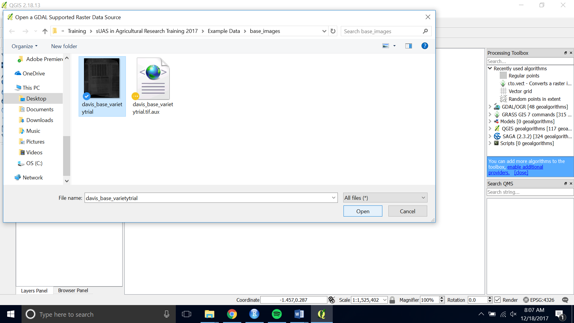
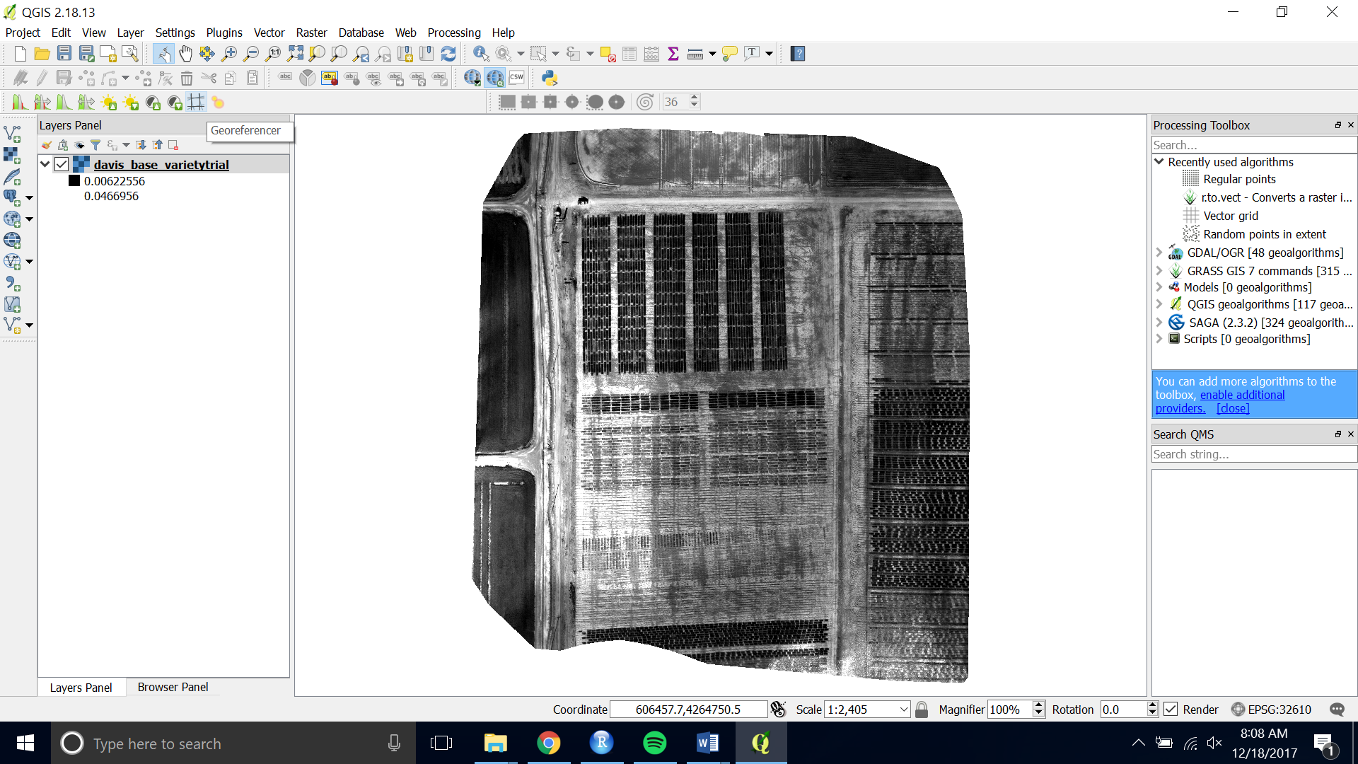
- Add a clearly captured GeoTIFF of our field: “Add Raster layer” (see figure 1)
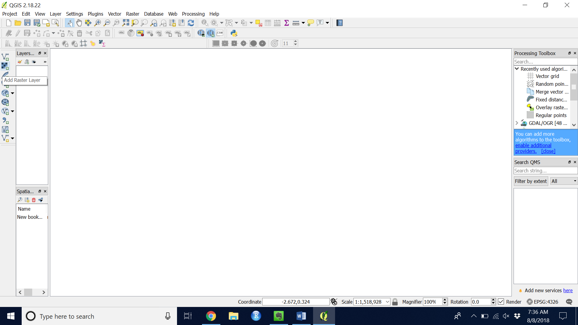 Figure 1.
 - Navigate to and choose your image file.
Shapefile Creation
- Create a new layer: “Layer” > “Create Layer” > “New Shapefile Layer…”
- Set the properties of your shapefile:
- Select “Point”
- Set the coordinate system to match your GeoTIFF (see Figures 2 & 3)
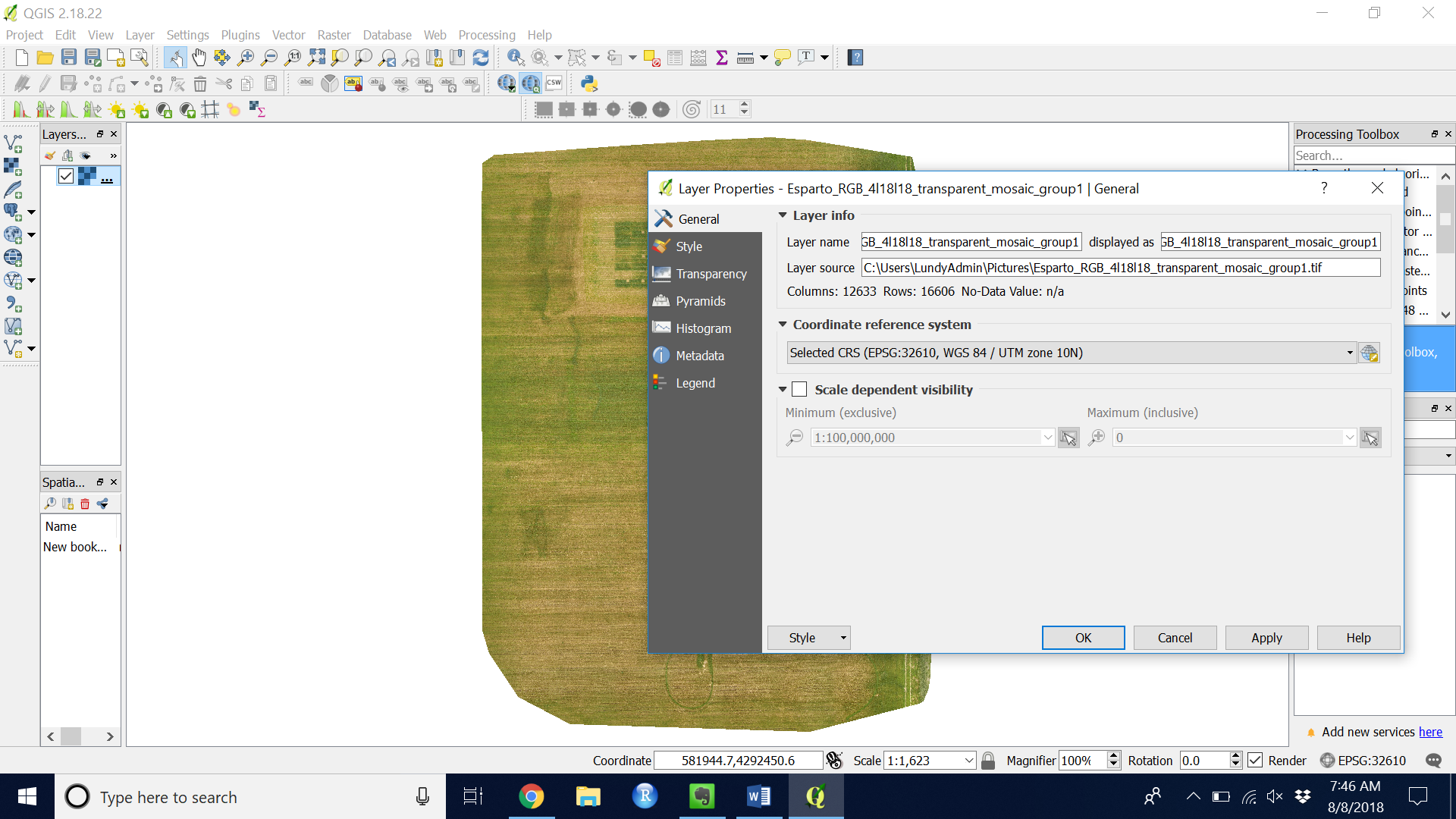 Figure 2. In the Layers panel, right click your GeoTIFF layer and add choose “Properties” to see the CRS.
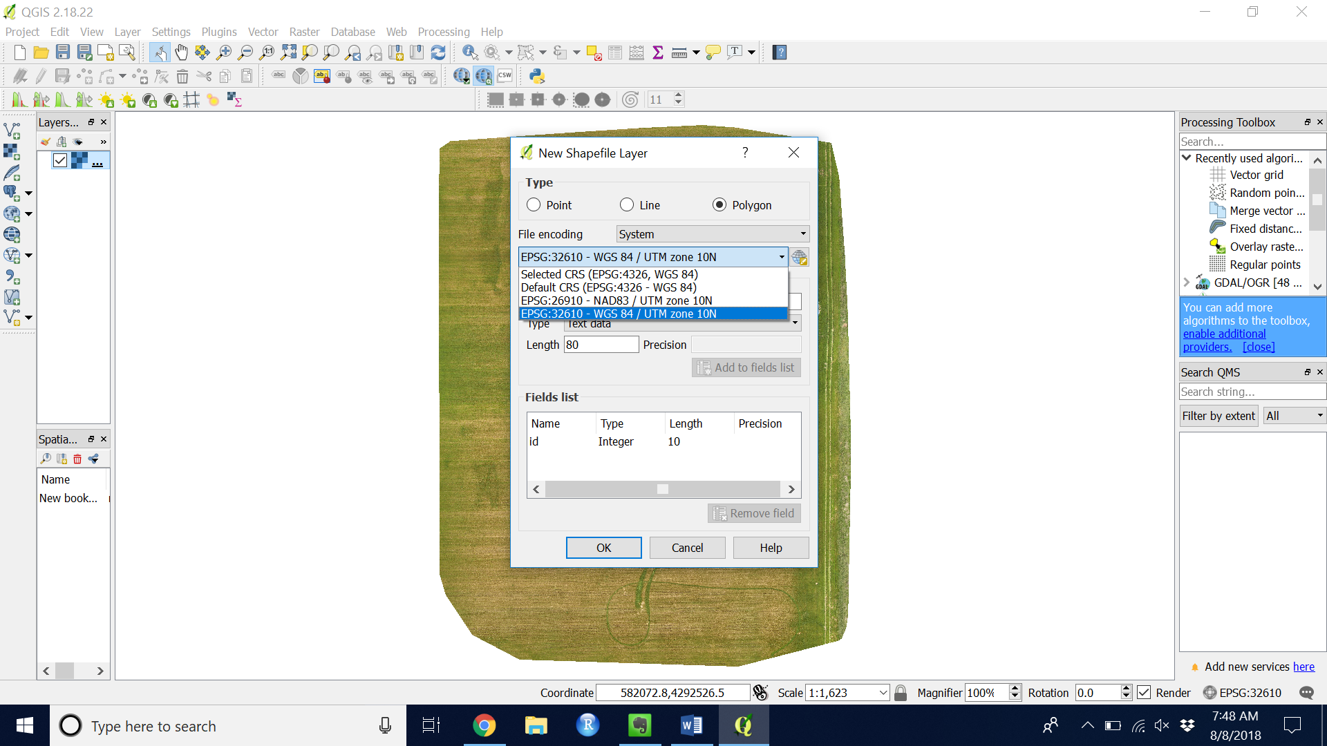 Figure 3. Choose the CRS that matches your GeoTIFF layer (WGS84/UTM zone 10N for most Northern California M100 flights)
- Click “OK”
- Name and save your shapefile when prompted.
- Edit the shapefile:
- Make sure the shapefile you created is highlighted in the layers panel.
- Toggle editing on by clicking the yellow pencil in the top left (see Figure 4)
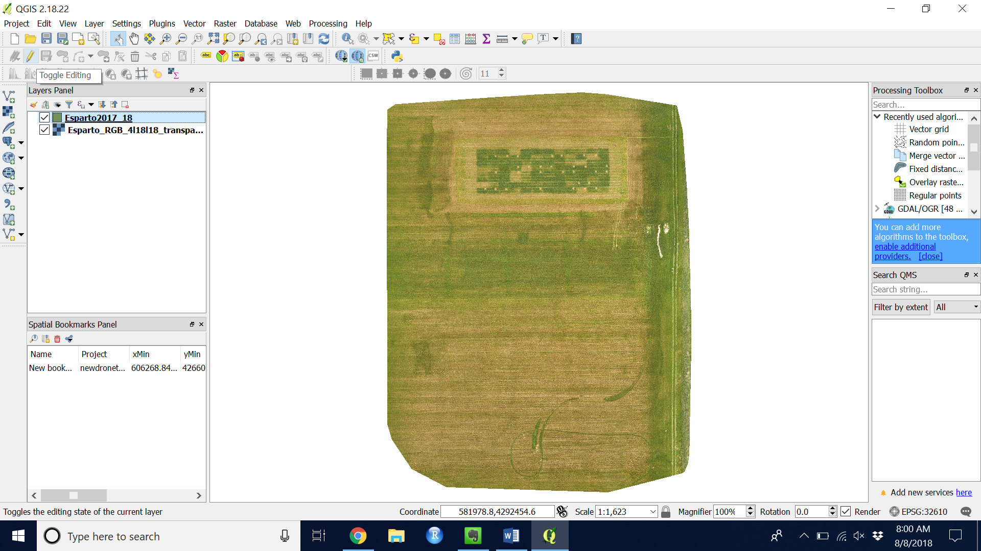 Figure 4. Add Feature to a shapefile
 - Add a feature by clicking the “Add feature” button (see Figure 5)
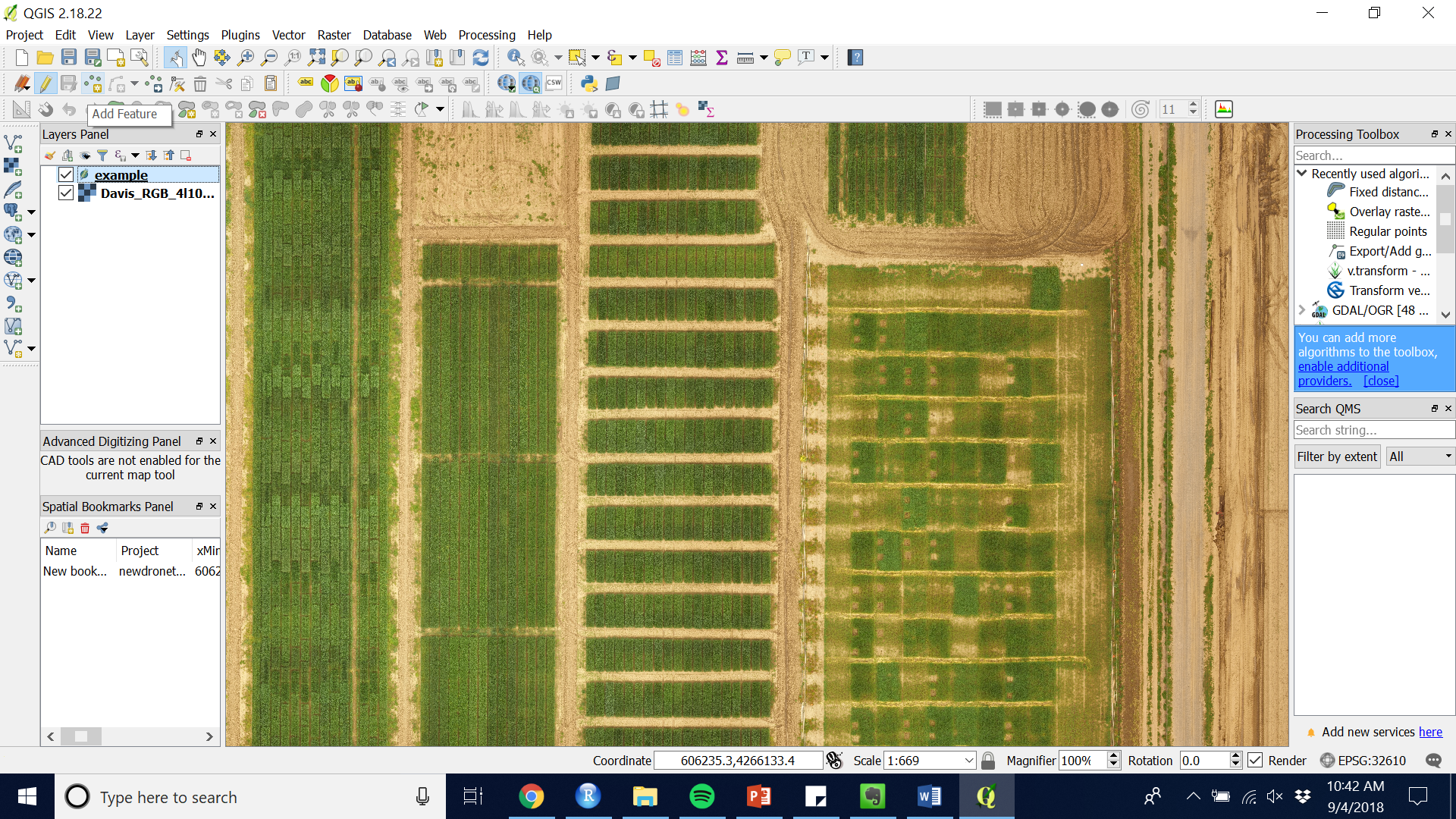 Figure 5.
 - Using your curser click a point at the center of each plot you wish to extract data from.
1. Make sure to create these points in order of plot number for easy data manipulation later.
- Set the ID of each point as a consecutive integer.
- Repeat for as many features as you desire for that image
- End your edit session by clicking the “Toggle Editing” button again.
- Save your edits when prompted.
- For rectangular buffers, use the rectBuffers.py custom script.
- Save “rectBuffers.py” in your “.qgis2\processing\scripts” folder 1. Copy located in \Box Sync\Grain Cropping Systems Lab\Drones
- In the processing toolbox open “Rectangular Buffers” under “Scripts” > “User scripts” (see figure 6).
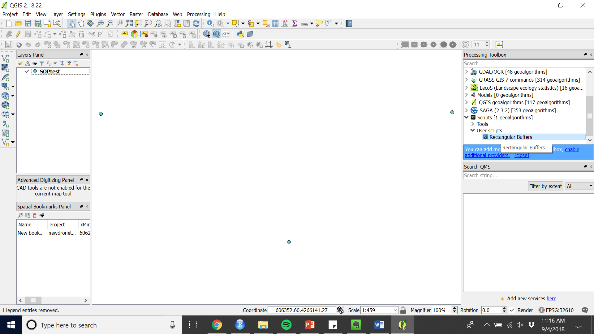 Figure 6. Run the custom script from the Processing Toolbox
 - Enter the height and width of your desired rectangle in meters (given that the projection is in UTM).
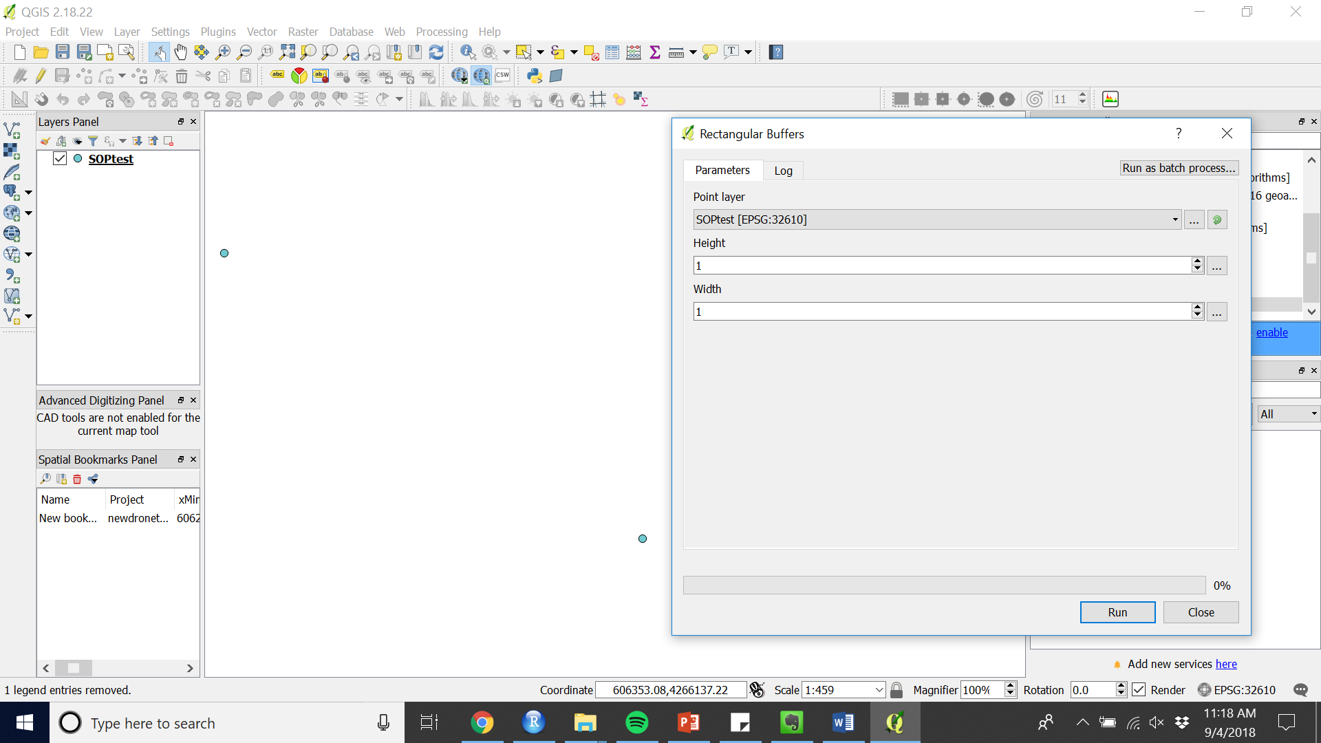 Figure 7. Enter the parameters for the extraction shapes in the Rectangular Buffers input
 - Add plot level metadata that can differentiate the plots by opening the Attribute table while editing is on.
- Ctrl + W to create a new field
- Name the new field appropriately and populate with metadata
- Save the rectangular_buffers shapefile by right clicking the layer and choosing “Save As…”
- For small grain variety trial images save shapefile as Location_Year. i.e. Davis_2018.shp
Georeferencing
With ground control points in Pix4D:
<https://support.pix4d.com/hc/en-us/articles/202558699-UsingGCPs#gsc.tab=0>
With tie points in QGIS:
- Open QGIS
- Project > New
- Add a raster layer of your base image.
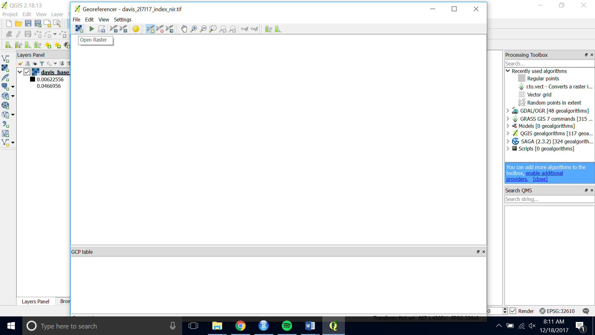
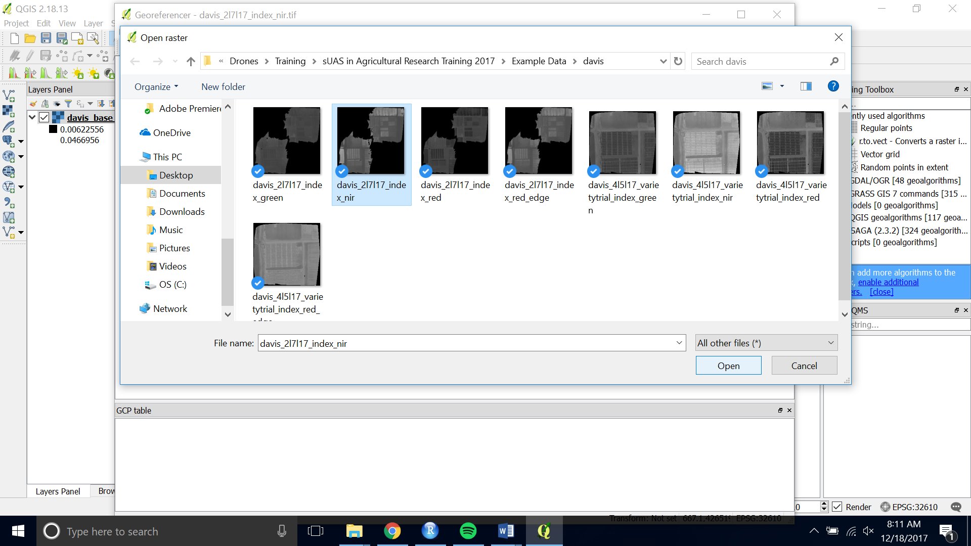
- Open the Georeferencer.
- Choose the raster you want to Georeference by opening the raster and navigating to the image you want to georeference
- Zoom and pan to a place in the image that will be there for the entirety of the season or the time period when you are planning to fly. Using the center of a plot works well.
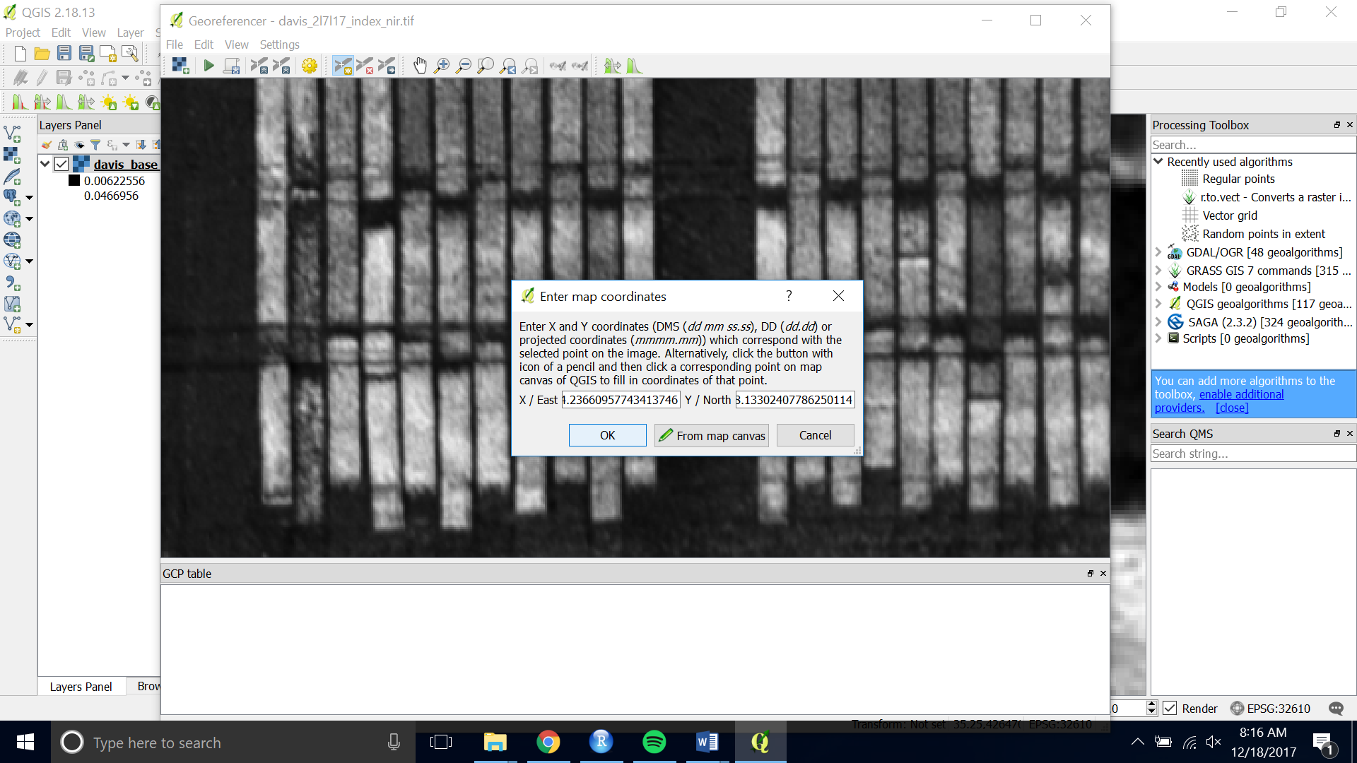
- Choose the yellow “Add Point” button at the top of the interface

- Click on the tie point you have chosen. Then choose “From Map Canvas”
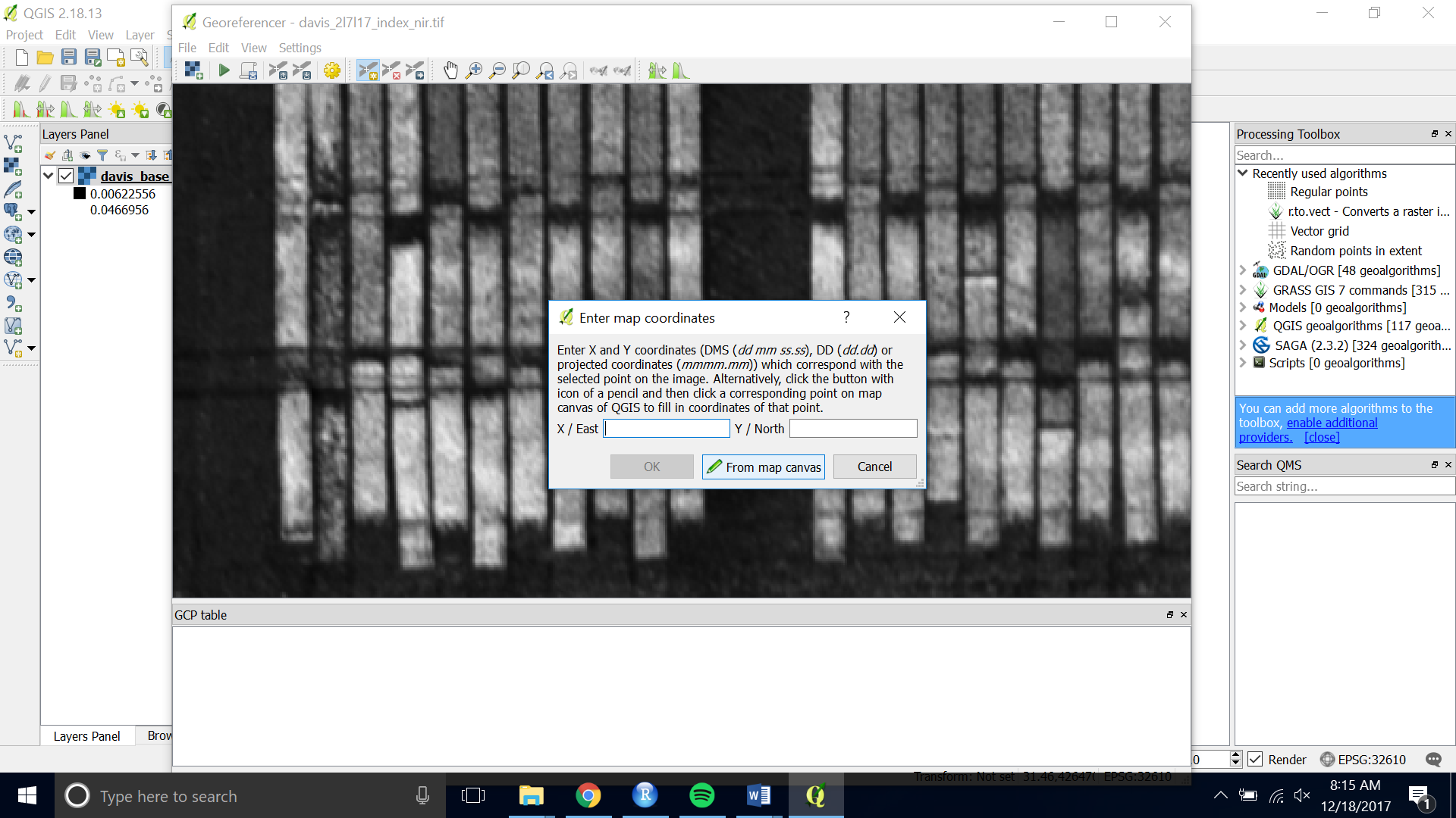
- Pan, zoom and click on the same point on the base image you loaded onto the map canvas.
- Then click “OK” to save the point.
- Do this for 5 – 10 points around your image.
- When you are satisfied with the number of ground control points, choose “ Start Georeferncing” (the green play button)
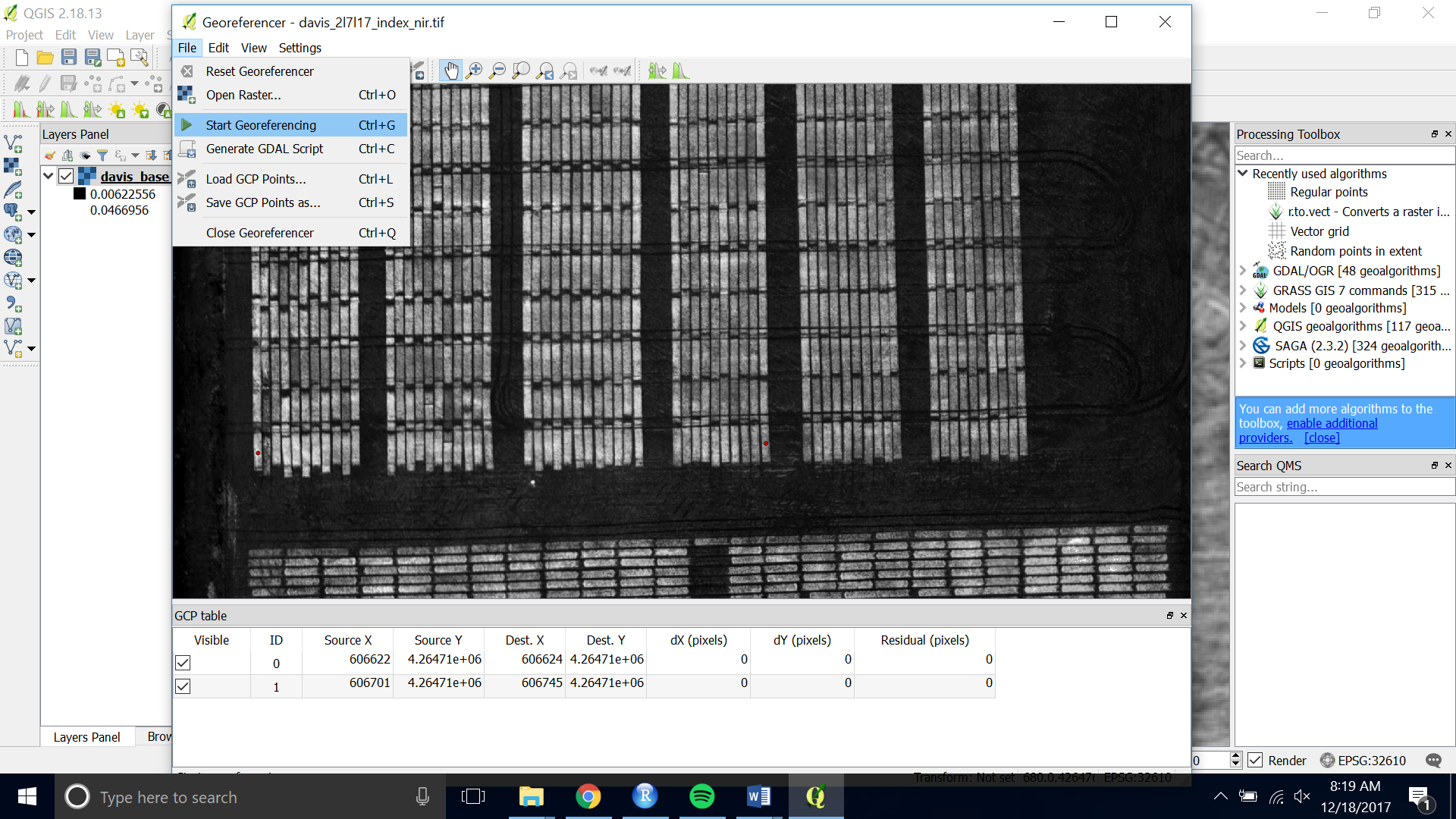
- If asked for the transformation information you can stick with the default. Check Load in QGIS when done and set the name of your output raster.
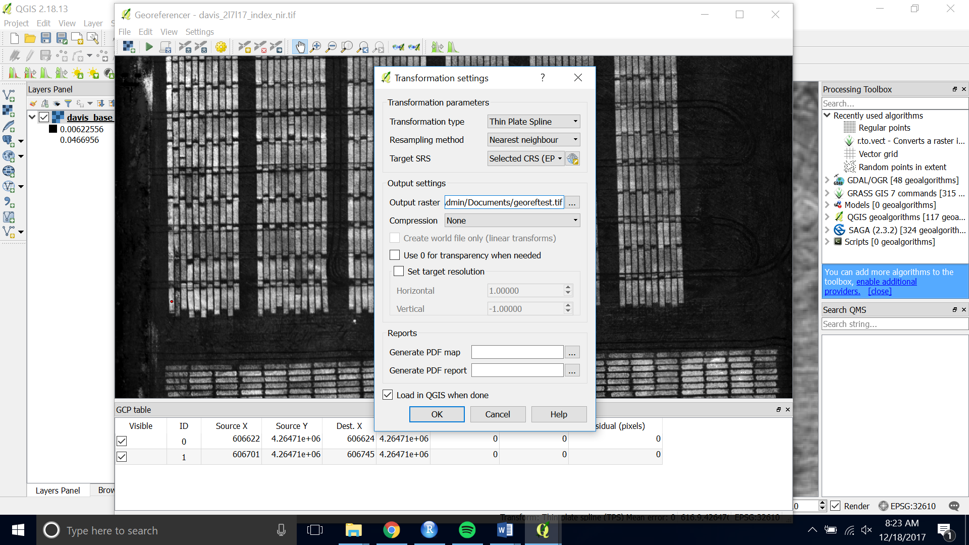
- Press the green “Start Georeferencing” button again. The georeferenced image will be saved and loaded onto the canvas.
- You can check that it aligns with your shapefile by loading the shapefile onto it.
Adjust Shapefile
- To adjust the shapefile, save the file with a new name.
- For small grain variety trial images save shapefile as Location_Date. i.e. Davis_4l3l2018.shp (those are the letter “L” between month, day, etc.)
- Toggle editing on for the new shapefile.
- Select all (or the subset that you wish to adjust) by choosing the “Select Features by area of single click” (see Figure 8) and drawing a rectangle around the features you want to adjust.
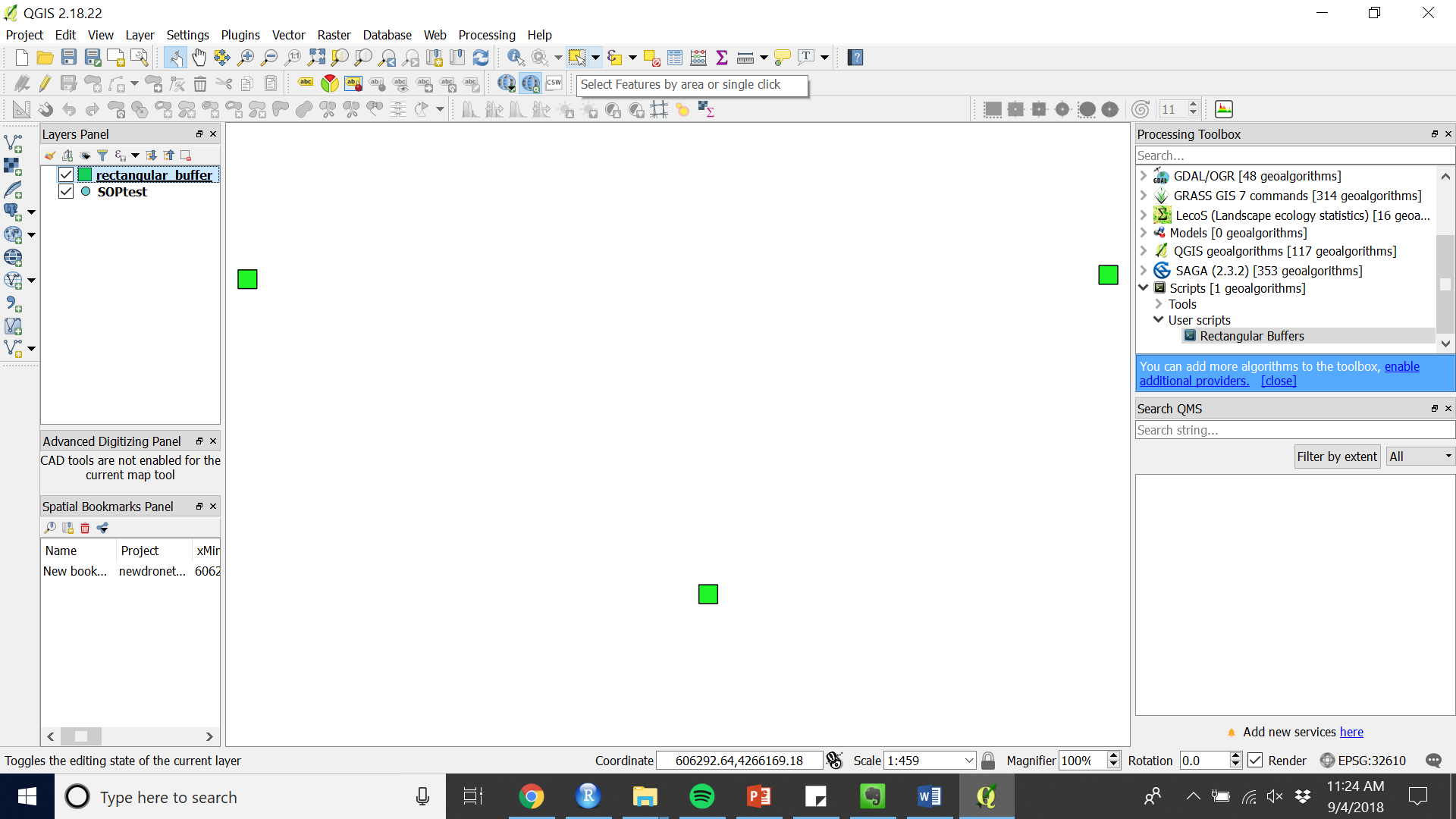 Figure 8. Select features tool
 - Move or rotate using the appropriate tools (see Figure 9 and 10).
 Figure 9. Move Feature(s)
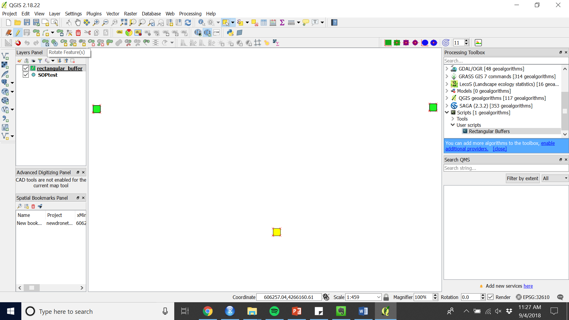 Figure 10. Rotate Feature(s)
 - Toggle editing off to save.
Value extraction
- Check the installation of the “Zonal statistics plugin”
- “Plugins” > “Manage and Install Plugins”
- Type Zonal Statistics in the search bar
- The “Zonal Statistics Plugin” should appear checked as in Figure 5.
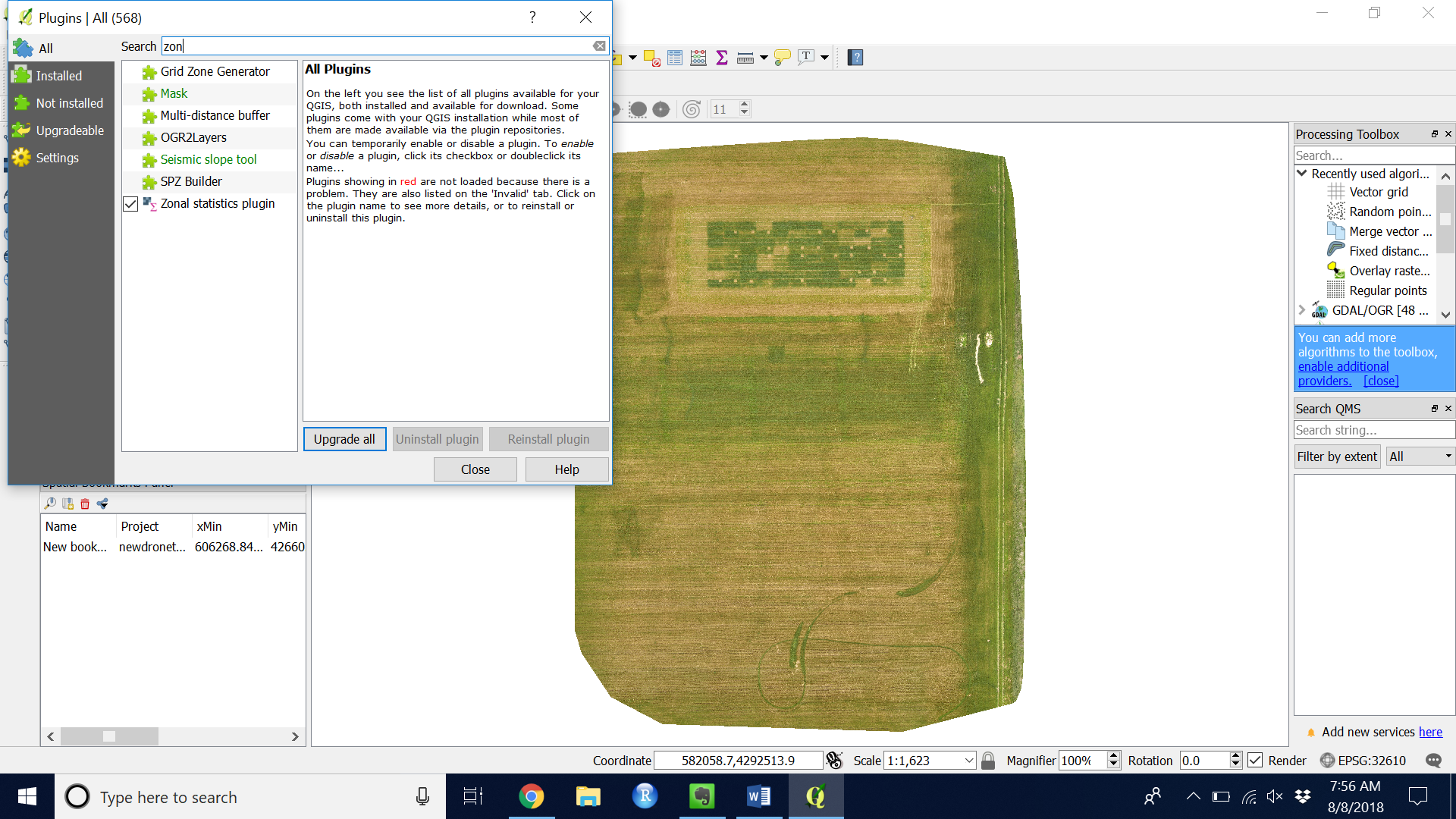 Figure 11. Zonal statistics plugin correct installation
 - Extract the image values using the “Zonal statistics plugin”
- Go to “Raster” > “Zonal statistics” > “Zonal statistics”
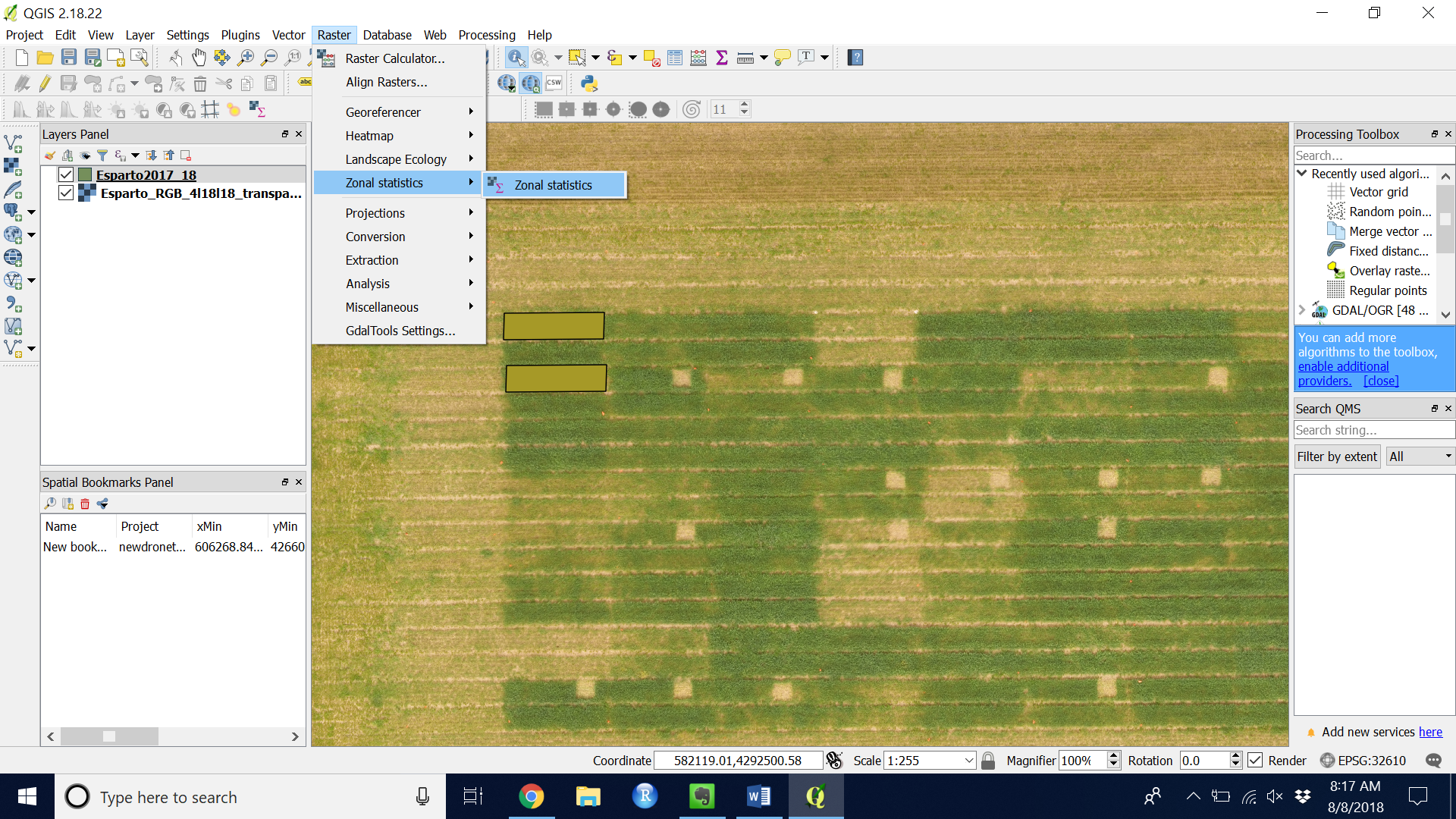 Figure 12. Navigating to the Zonal statistics plugin
 - Choose the polygon layer and the band you wish to extract.
- Check whichever boxes you want data for, e.g. “mean”, “median”, “mode”, “standard deviation”, “minimum”, and “maximum”.
1. For small grain variety trial images set the prefix to match the band i.e. “blue_”, “green_”, “nir_”, “edge_”
- Shapefile column names have a limited number of characters so follow these exactly. 1. Check “mean”, “median”, “standard deviation”, “minimum”, and “maximum”
- Click “OK” to run the algorithm
- For small grain variety trial images repeat for each band (should be a blue, green, nir, and red edge band)
- Look at the values you extracted by right clicking on your shapefile layer and navigate to “Open Attribute Table” (see Figures 13 & 14)
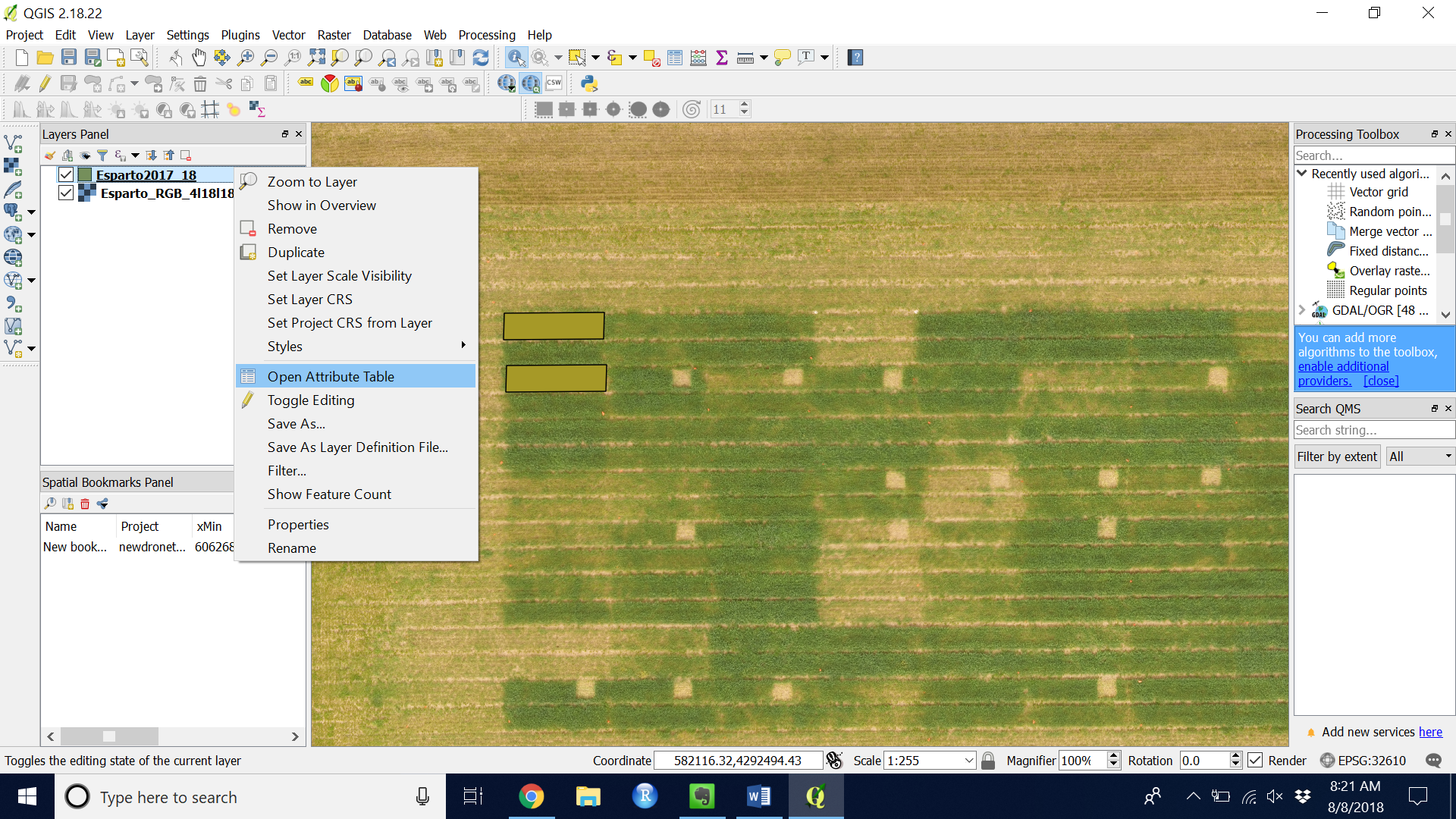 Figure 13. Navigate to Attribute Table
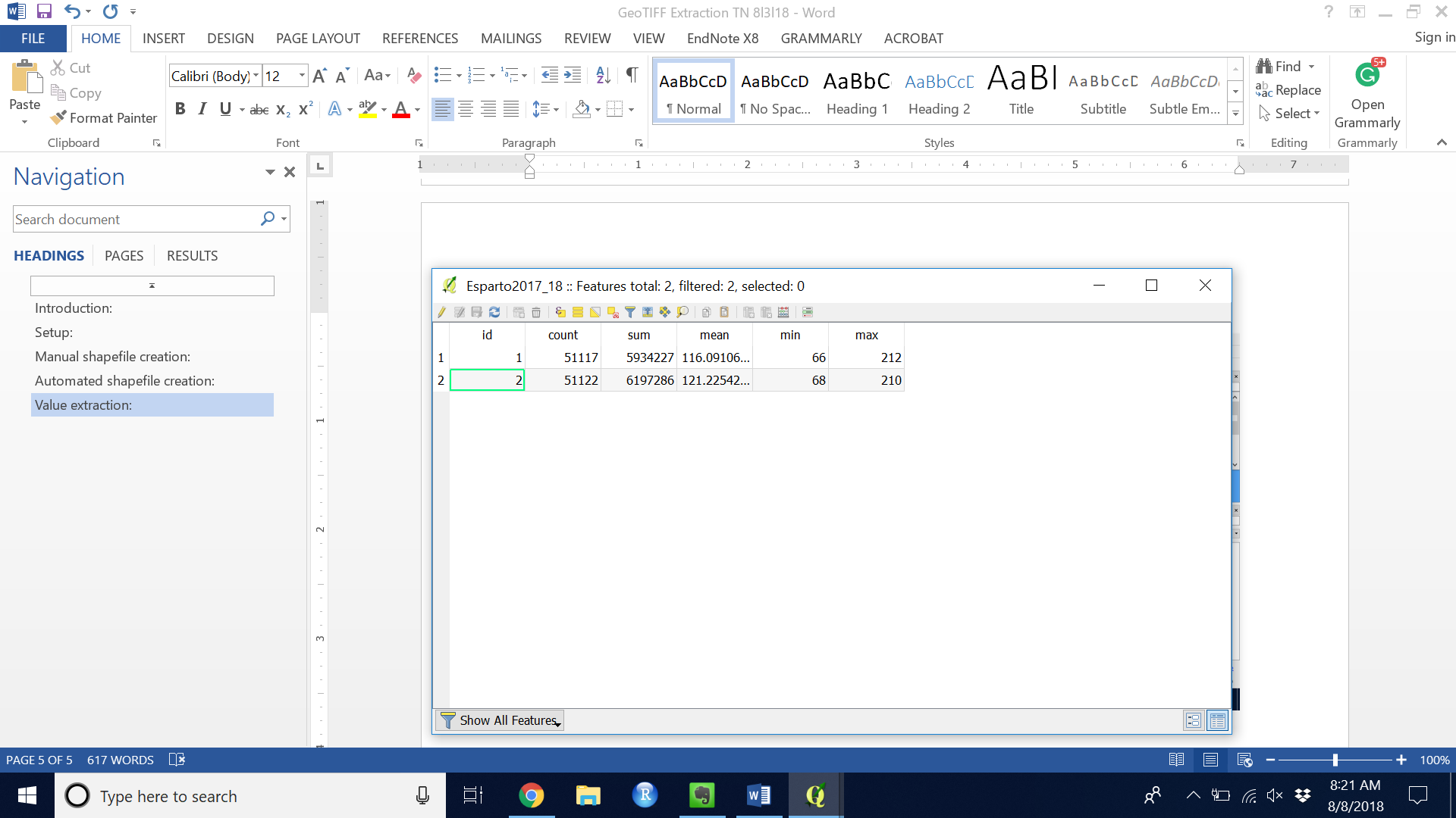 Figure 14. Example Attribute Table
 - Save the shapefile and close QGIS
Value Analysis
To open table in Excel:
Make sure to QGIS is closed.
Open Microsoft Excel
Choose “Open Other Workbooks” or “File” > “Browse”
Navigate to the file where you saved your shapefile
Make sure “All files” is selected in drop-down list at bottom right, NOT “All excel files”
Select the .dbf file you just saved
To open the attribute table in R use the following code below. Adjust the file path accordingly.
filepath <- "C:/Users/LundyAdmin/Documents" library(foreign) read.dbf(file.path(filepath, "Esparto2017_18.dbf"))